PET bottle manufacturing looks like one of the most approachable entries into plastics processing. The process is well understood, the equipment is mature, the raw material is a global commodity, and demand for packaged water and beverages grows almost everywhere. That surface simplicity is exactly why so many PET bottle factory investment projects disappoint. Two plants can install identical stretch blow molding lines in the same month, buy preforms of the same grade, and end up with payback periods that differ by a factor of four. One recovers its invested capital in about fourteen months. The other is still waiting after five years.

The difference almost never comes from the machine. It comes from five operational variables that most feasibility studies treat as assumptions rather than as risks: capacity utilization, scrap rate, energy tariff level, customer concentration, and product mix. Each of these is a distribution, not a number, and each of them compounds with the others. A plant running at 55 percent utilization with a 4 percent scrap rate and a single dominant customer is not slightly worse than a plant at 85 percent utilization with 1.2 percent scrap and four balanced customers. It is a fundamentally different business with a fundamentally different payback profile.

YuDa Machinery, a Wanplas factory with more than twenty years of specialization in PET bottle blow molding machines, exports to over sixty countries and holds more than twenty patents in stretch blow molding technology. Across those installations, one pattern repeats: the projects that hit their payback targets are the ones that modeled utilization and scrap honestly before they signed anything. This guide sets out the framework they used. Every figure in it is expressed as a ratio, a percentage, a physical unit, or an index relative to a stated baseline, so that it stays valid regardless of region or year, and so that the structure of the decision remains visible rather than buried under project-specific numbers.

Why Payback Modeling Fails in PET Bottle Projects

Most PET bottle factory payback models fail in the same three places, and all three failures push the projected payback period in the optimistic direction. Recognizing them early is the single highest-return activity in project preparation, because a model that is wrong by 40 percent on the revenue side cannot be rescued by any amount of operational discipline later.

Error One: Treating Nameplate Output as Actual Output

A machine rated at 12,000 bottles per hour does not produce 12,000 saleable bottles in any real hour of any real week. Nameplate output is a mechanical rating measured under laboratory conditions: one bottle format, one preform lot, a fully warmed oven, no changeovers, no preform feed interruptions, no cap or label starvation downstream, and no quality holds. What the plant actually earns is governed by overall equipment effectiveness, the product of availability, performance rate, and quality rate.

In PET stretch blow molding, availability losses come from mold changeovers, preform hopper starvation, air compressor trips, chilled water excursions, and planned maintenance. Performance losses come from running below rated speed to hold wall distribution on a marginal preform, from oven ramp-up after every stop, and from micro-stops at the transfer star or the discharge conveyor. Quality losses come from wall thickness deviation, base clearing failures, neck deformation, and burst failures on pressure test.

A mature PET bottle plant with a stable SKU set, disciplined changeover practice, and reliable utilities typically achieves overall equipment effectiveness in the 75 to 82 percent band. A well-run plant on a single high-volume water format can reach 85 to 88 percent. A new plant in its first year, or any plant running a fragmented SKU portfolio, commonly lands between 60 and 72 percent. Building a revenue model on nameplate output therefore overstates saleable volume by roughly 20 to 40 percent before a single other error is made. That error alone can move a projected 18-month payback to a real 30-month payback.

Error Two: Underweighting the Preform and Resin Share

The second failure is structural. Many first-time investors mentally model a bottle plant as a machinery business, so they scrutinize machine specifications, electricity consumption, and headcount, and treat material as a pass-through. In reality, preform or resin accounts for roughly 62 to 72 percent of total conversion cost in a typical water or carbonated soft drink bottle operation. Everything else combined, including electricity, labor, depreciation, mold amortization, maintenance, logistics, and overhead, sits in the remaining 28 to 38 percent.

This has a hard consequence for improvement priorities. A 10 percent reduction in electricity consumption improves total conversion cost by roughly 0.6 to 1.2 percent. A 10 percent reduction in labor improves it by roughly 0.4 to 0.9 percent. But a reduction in scrap rate from 4 percent to 1.5 percent improves it by roughly 1.6 to 1.8 percent on material alone, and simultaneously increases saleable output, which improves the fixed-cost absorption on every remaining line item. Yield is the highest-leverage lever in a PET bottle plant, and it is the one most often delegated to the least experienced shift.

Error Three: Ignoring the Ramp-Up Trough

The third failure is temporal. Payback models frequently assume that revenue begins in month one at steady-state volume. Real PET bottle projects go through a ramp-up period of three to six months during which utilization climbs from roughly 15 to 25 percent in the commissioning month toward 70 to 85 percent, while scrap falls from 6 to 10 percent toward 1.5 to 2.5 percent. During that window the plant consumes working capital rather than generating it: preform inventory builds, spare parts are stocked, operators are trained on paid time, mold trials burn material, and customers withhold volume until first-article approval is granted.

The cumulative cash absorption of a normal ramp-up is not trivial, and it does not appear as an investment line item in most spreadsheets. It appears as a delay. A project that assumes month-one steady state and actually experiences a five-month ramp will show a payback period roughly four to seven months longer than modeled, purely from the timing shift, before any operational shortfall is considered.

Cost Structure Anatomy of a PET Bottle Plant

Understanding where value leaks in a PET bottle plant requires a share-based view of conversion cost rather than an absolute one. The table below gives typical share bands for a stretch blow molding operation producing standard water and beverage bottles from purchased preforms, running two or three shifts. Shares shift with bottle weight, energy tariff level, and labor intensity, but the ranking of the line items is remarkably stable across regions.

Table 1 — Typical conversion cost structure of a PET bottle plant (share of total, purchased-preform model)

Cost element	Share of total	Behavior	Primary driver	Improvement leverage
Preform / resin	62–72%	Variable	Bottle gram weight, scrap rate, resin grade	Very High
Electricity	6–12%	Semi-variable	Oven design, air recovery, tariff band	Medium
Direct labor	4–9%	Semi-fixed	Automation level, shift pattern, SKU count	Medium
Depreciation	5–10%	Fixed	Capital intensity, utilization	Low (set at purchase)
Mold amortization	2–4%	Fixed per SKU	SKU count, mold life, changeover frequency	Medium
Maintenance and spares	1–3%	Semi-variable	Machine generation, preventive discipline	Medium
Outbound logistics	3–6%	Variable	Delivery radius, load factor, bottle volume	High
Plant overhead	3–5%	Fixed	Facility size, administration, quality function	Low

Three conclusions follow directly from this structure, and each of them contradicts a common instinct.

First, saving material beats saving energy and labor combined. Electricity and labor together occupy 10 to 21 percent of conversion cost. Even an aggressive, well-executed program that cuts both by a fifth improves total cost by about 2 to 4 percent. Cutting scrap from 4 percent to 1.5 percent, by contrast, recovers 1.5 to 1.8 percent on material and lifts saleable output by roughly 2.6 percent, which then improves the absorption of every fixed line item. The combined effect typically exceeds the energy-plus-labor program while requiring far less capital.

Second, depreciation only becomes a problem at low utilization. At 85 percent utilization, depreciation at 5 to 10 percent of conversion cost is comfortably absorbed. At 45 percent utilization, the same absolute depreciation lands on roughly half as many bottles, so its share can double to 12 to 20 percent, and the plant may find itself structurally unable to compete on price with a fully loaded competitor running identical equipment. Utilization, not capital intensity, is what makes depreciation dangerous.

Third, logistics is a bigger lever than most operators assume. At 3 to 6 percent, outbound freight for empty bottles rivals electricity. Because empty PET bottles have extremely low bulk density, a truck is effectively transporting air, and every additional 100 km of delivery radius adds meaningfully to unit cost without adding any value the customer perceives. Location decisions made for land availability rather than for customer proximity can quietly consume a full margin point per year for the life of the plant.

The Five Variables That Decide Payback

Once the cost structure is understood, the payback question reduces to five variables. These are the only inputs that move the answer by more than a few months, and they interact multiplicatively rather than additively. A plant that is mediocre on all five is not mediocre overall; it is unviable.

Variable 1: Capacity Utilization

Capacity utilization is the master variable because it simultaneously scales revenue and dilutes fixed cost. It is determined less by machine capability than by order book quality. Utilization is the physical expression of commercial performance: a plant with three balanced annual contracts and a seasonal buffer customer will run at 80 to 88 percent, while a plant selling into a spot market will oscillate between 35 and 70 percent depending on the month.

The practical implication is that equipment sizing should follow the contracted portion of demand, not the hoped-for portion. Installing a 15,000 bottle-per-hour line against 45 million bottles of contracted annual volume guarantees structural under-utilization; installing a 7,000 bottle-per-hour line against the same volume and adding a second line when contracts mature produces a shorter payback despite the higher unit conversion cost of the smaller machine.

Variable 2: Scrap Rate

Scrap rate acts directly on the largest cost element. In stretch blow molding, scrap arises from oven profile errors producing uneven wall distribution, preform lots with inconsistent intrinsic viscosity or moisture, mold temperature drift, transfer damage at the neck, base clearing failures on petaloid designs, and contamination during regrind handling. A disciplined plant with a stable preform supply and a documented oven recipe per SKU holds scrap in the 0.8 to 1.8 percent range. A plant with unstable preforms, undertrained operators, or an over-fragmented SKU portfolio routinely runs 4 to 8 percent.

Variable 3: Energy Tariff Level

Energy tariff level is largely outside the operator’s control but entirely inside the investor’s location decision. Because electricity is 6 to 12 percent of conversion cost, moving from a low tariff band to a high tariff band can add 4 to 8 percent to total cost, which for a thin-margin water bottle business can consume half the gross margin. Tariff structure matters as much as tariff level: plants in regions with time-of-use pricing can shift oven-heavy production into off-peak windows and recover several months of payback simply by rescheduling shifts.

Variable 4: Customer Concentration

Customer concentration is the risk variable that does not show up in the base-case model at all, because in the base case the customer stays. Its effect is entirely on the downside distribution. A plant where a single customer represents more than 50 percent of volume has effectively financed its equipment against a single commercial relationship. When that customer renegotiates, insources, or shifts to a competing supplier, utilization does not fall gradually; it steps down, and payback extends by years rather than months.

Variable 5: Product Mix

Product mix determines the gross margin band the plant can access and the changeover burden it must carry. Water bottles are high-volume and thin-margin. Carbonated soft drink bottles require petaloid base geometry and tighter process control, and carry a middle margin. Hot-fill bottles require heat-set molds, crystallized necks, and higher machine capability, and command the highest margin per bottle. Daily chemical and edible oil containers are small-batch, multi-format, high-margin, but changeover-intensive. A plant that mixes these categories deliberately can lift blended margin substantially; a plant that mixes them accidentally destroys utilization through changeover losses.

Sensitivity Analysis: How Utilization Drives Payback

Capacity utilization is the variable with the steepest gradient in the entire model, and its effect is non-linear. Below roughly 55 percent, fixed cost absorption deteriorates fast enough that gross margin can turn negative even with perfect operational discipline. Above roughly 85 percent, the returns to further utilization flatten because overtime premiums, accelerated wear, and compressed maintenance windows begin to offset the volume gain.

The table below indexes effective annual output and unit conversion cost against an 85 percent utilization baseline, defined as 100 index points. Payback ranges assume a purchased-preform model, a stable two-SKU portfolio, a medium energy tariff band, and a scrap rate of 1.5 percent, so that utilization is the only variable moving.

Table 2 — Utilization sensitivity (baseline: 85% utilization = 100 index points)

Capacity utilization	Effective annual output index	Unit conversion cost index	Gross margin band	Payback period range	Business condition
40%	47	141	Negative to 3%	Beyond 72 months or not achieved	Structurally unviable
55%	65	122	3–8%	46–72 months	Survival mode
70%	82	109	9–15%	29–44 months	Acceptable, improvable
85%	100	100	16–24%	19–28 months	Target operating state
95%	112	96	20–28%	14–23 months	Excellent, capacity-constrained

Read this table as a warning about equipment sizing rather than as an encouragement to buy the fastest machine available. The 95 percent row is not reachable by installing a faster line; it is reachable only by matching installed capacity to genuinely contracted volume. An oversized line pushes the plant into the 40 or 55 percent rows, where the unit conversion cost penalty of 22 to 41 index points swamps any per-bottle efficiency advantage the high-speed machine offered in the first place.

Two secondary observations are worth extracting. First, the gap between the 70 percent row and the 85 percent row is worth roughly 10 to 16 months of payback, which is usually larger than the entire difference between two competing machine specifications. Second, the movement from 55 percent to 70 percent is worth more than the movement from 85 percent to 95 percent, meaning that recovery effort on an under-loaded plant returns more than optimization effort on a well-loaded one. Commercial work outperforms engineering work when utilization is the binding constraint.

How to Build a Defensible Utilization Assumption

A defensible utilization assumption is constructed bottom-up from four components rather than asserted top-down. Start with calendar hours available under the intended shift pattern. Subtract planned maintenance, statutory holidays, and annual shutdown. Apply a changeover allowance derived from the planned SKU count and realistic changeover duration — a full mold and neck-format change on a linear stretch blow molding machine typically takes 45 to 120 minutes depending on cavity count and whether the neck finish changes. Then apply a performance factor for oven ramp, micro-stops, and speed derating, and a quality factor equal to one minus the expected scrap rate.

A plant running four SKUs with two changeovers per week, a 90-minute average changeover, three shifts, and a 1.5 percent scrap rate will land near 78 to 83 percent in a mature year. The same plant running twelve SKUs with eight changeovers per week will land near 62 to 68 percent, all else equal. That 15-point spread is the difference between a 24-month payback and a 38-month payback, and it is decided by the sales team’s SKU acceptance policy, not by the machine.

Scrap Rate: The Silent Payback Killer

Scrap is the most underestimated variable in PET bottle economics because its accounting treatment hides its true impact. A plant reporting 3 percent scrap tends to think it has lost 3 percent of something. In fact it has lost 3 percent of the largest cost element, plus the energy already invested in heating those preforms, plus the machine time that produced them, plus the fixed cost that must now be recovered from fewer good bottles, plus the handling and regrind cost of the rejects themselves. The compounded effect is several times the headline number.

The table below indexes those effects against a 0.5 percent scrap baseline set at 100 index points. Material loss index tracks the value of resin permanently downgraded or lost. Rework and regrind energy index tracks the additional electrical and handling burden of processing rejects. Effective good output index shows saleable volume relative to the baseline at identical machine hours.

Table 3 — Scrap rate sensitivity (baseline: 0.5% scrap = 100 index points)

Scrap rate	Material loss index	Rework / regrind energy index	Effective good output index	Added payback months	Typical root cause profile
0.5%	100	100	100	Baseline	Mature process, single stable SKU, validated preform lot
1.5%	300	240	99.0	+2 to +4	Normal multi-SKU operation with documented oven recipes
3.0%	600	460	97.5	+5 to +9	Preform lot variation, drifting mold temperature control
6.0%	1200	880	94.5	+12 to +20	Untrained shift, poor changeover discipline, marginal air supply
10.0%	2000	1450	90.5	+24 to +40	Unstable preform sourcing, uncontrolled process, no statistical process control

Where Scrap Actually Originates in Stretch Blow Molding

Effective scrap reduction requires knowing which of the six dominant mechanisms is active, because the countermeasures do not overlap.

• Oven profile error. Uneven axial temperature distribution in the preform produces wall thickness deviation, thin shoulders, or thick bases. The countermeasure is a documented lamp-zone recipe per preform geometry, verified with a wall thickness map on start-up and after every changeover.
• Preform condition. Intrinsic viscosity drift between resin lots, excessive moisture, acetaldehyde variation, or crystallinity in the neck from over-drying all change the stretch behavior. The countermeasure is incoming inspection with intrinsic viscosity and moisture verification, plus a preform conditioning period at controlled ambient temperature before processing.
• Stretch rod and pre-blow timing. Incorrect stretch rod speed or pre-blow onset produces off-center bases and unbalanced material distribution. The countermeasure is servo-controlled stretch with recipe storage, so timing is restored exactly after every stop.
• Mold temperature drift. Chilled water temperature excursion changes the frozen layer formation rate and the base clearing behavior. The countermeasure is a closed-loop mold temperature circuit with alarm limits, not a shared chilled water header serving unrelated loads.
• Neck and transfer damage. Gripper wear, misaligned star wheels, and neck support ring deformation cause leaks at capping. The countermeasure is a scheduled gripper inspection interval and neck ring gauging.
• Air supply instability. Pressure sag in the high-pressure circuit during peak demand produces incomplete blowing and inconsistent base definition. The countermeasure is correctly sized receiver volume and a compressor control strategy that anticipates blow demand rather than reacting to it.

Notice that four of the six countermeasures are procedural rather than capital. Scrap reduction is one of the very few improvement levers in a PET bottle plant that shortens payback without lengthening it first.

Energy Consumption Modeling

Electricity is the second largest controllable cost in a PET bottle plant, and unlike material cost it is almost entirely determined by equipment design decisions made at purchase. Once an oven architecture and an air system are installed, the plant’s energy intensity is largely fixed for the life of the asset. Understanding the split before purchase is therefore worth more than any retrofit afterwards.

Where the Energy Goes

In a modern stretch blow molding line, total electrical demand divides into three blocks with remarkably consistent proportions:

• Infrared heating lamps: 55–65%. The oven raises preform body temperature to the orientation window, typically 95 to 115 degrees Celsius depending on resin and bottle geometry. Lamp efficiency, reflector design, lamp-to-preform distance, and zone control determine how much of that energy reaches the preform rather than the surrounding air.
• High-pressure air: 25–35%. Blowing air at 3.0 to 4.0 MPa is the second block. Air consumption scales with bottle internal volume and with the number of blow cycles per hour, and compression is thermodynamically expensive, which is why air recovery has such a strong effect on the total.
• Servo drives and mechanical systems: 5–10%. Clamping, transfer, stretch rod actuation, conveying and chilled water pumping make up the remainder. Servo-driven architectures consume less than hydraulic equivalents and, more importantly, consume proportionally to actual motion rather than continuously.

Because heating dominates, the single most influential design parameter in the entire energy model is the geometry of the heating oven. YuDa’s FGX series minimizes heater-to-preform distance to 38.1 mm, which increases the share of radiant energy actually absorbed by the preform rather than lost to the oven enclosure and the cooling air. In comparison with conventional heating oven layouts, this configuration reduces heating electricity consumption by more than 30 percent, and because heating is 55 to 65 percent of the total, that translates into roughly 17 to 20 percent off total line electricity.

Energy Intensity by Bottle Format

The practical unit for benchmarking is kilowatt-hours per 1,000 bottles, measured at the line boundary and including the high-pressure compressor. The table below gives typical bands for a servo-driven line with a modern oven, running at normal utilization. Older-generation lines with wide heater spacing and no air recovery typically run 25 to 45 percent above these bands.

Table 4 — Energy intensity by bottle format (servo line, modern oven, compressor included)

Bottle format	Typical preform weight	Energy intensity	Heating share	Air share	Notes
200–350 mL still water / dairy	9–14 g	12–18 kWh / 1,000 bottles	58–64%	24–30%	Lowest intensity; high cycle count
500 mL still water	11–16 g	15–22 kWh / 1,000 bottles	57–63%	26–32%	Highest-volume global format
600 mL–1.0 L water / juice	18–24 g	22–30 kWh / 1,000 bottles	56–62%	27–33%	Longer oven dwell required
1.5 L still water	28–36 g	30–40 kWh / 1,000 bottles	55–61%	28–34%	Air volume rises faster than heating
2.0 L carbonated soft drink	42–52 g	42–56 kWh / 1,000 bottles	54–60%	30–36%	Petaloid base; higher blow pressure
5 L bulk water	90–110 g	80–105 kWh / 1,000 bottles	53–59%	31–37%	Low cycle count, high per-unit energy

Three Energy Measures and Their Payback Contribution

Three interventions dominate the achievable energy improvement, and each can be expressed as a contribution to payback shortening rather than as an abstract percentage.

Air recovery systems capture exhaust air from the blowing station and return it to the pre-blow circuit or to the plant’s low-pressure network. Recovery of 30 to 40 percent of high-pressure air consumption is achievable on standard water bottle formats. Because air is 25 to 35 percent of line energy and energy is 6 to 12 percent of conversion cost, a well-implemented recovery system improves total conversion cost by roughly 0.5 to 1.5 percent, which on a well-loaded plant shortens payback by approximately 1 to 3 months net of the additional capital involved.

Zoned infrared lamp control allows the oven to switch off or derate lamp banks not required by the current preform geometry, and to hold different power profiles for different axial zones. On multi-SKU plants this both reduces energy and improves wall distribution, so it contributes to scrap reduction simultaneously. Typical contribution is 0.5 to 2 months of payback shortening, weighted toward plants with fragmented portfolios.

Preform preheating and conditioning discipline is the least capital-intensive of the three. Preforms entering the oven at a stable, controlled ambient temperature require less oven correction and produce less startup scrap after every stop. Plants that move preform storage from an unconditioned yard to a temperature-stable indoor area frequently see both scrap and oven power fall. Contribution is modest in energy terms but meaningful once the scrap effect is included, generally 0.5 to 1.5 months.

Taken together, a disciplined energy program contributes roughly 2 to 6 months of payback shortening. That is real and worth pursuing, but it should be read alongside the scrap table above, where moving from 6 percent to 1.5 percent scrap is worth 12 to 20 months. Energy is a good second priority. It is a poor first priority.

Equipment Capital Intensity Comparison

Equipment selection determines two things simultaneously: how much capital must be recovered, and how efficiently each bottle can be produced. These pull in opposite directions, which is why there is no universally correct machine tier. The table below indexes capital intensity against a semi-automatic 1,000 to 2,000 bottle-per-hour installation set at 100 baseline index points. Unit conversion cost index assumes each tier is operating at its own appropriate volume band with 85 percent utilization; it is not comparable across tiers at equal volume.

Table 5 — Equipment tier comparison (baseline: semi-automatic 1,000–2,000 BPH = 100 capital intensity index points)

Equipment tier	Capital intensity index	Line footprint	Operators per shift	Energy intensity index	Unit conversion cost index	Suitable annual volume band
Semi-automatic, 1,000–2,000 BPH	100 (baseline)	20–28 m²	3–4	145	163	Up to 8 million bottles
Standard automatic, 4,000 BPH	215–255	30–38 m²	2	112	118	8–25 million bottles
Standard automatic, 7,000 BPH	285–335	38–46 m²	2	104	106	25–45 million bottles
High-speed FGX, 10,000 BPH	380–450	46–58 m²	2	96	94	45–70 million bottles
High-speed FGX, 15,000 BPH	520–620	58–72 m²	2	92	88	70–105 million bottles

The critical reading is the relationship between the second column and the last column. Capital intensity rises roughly five to six fold from the semi-automatic tier to the top high-speed tier, while unit conversion cost falls by about 46 percent. That trade is favorable only if the volume band is actually filled. A 15,000 bottle-per-hour line running at 40 percent utilization has a worse unit conversion cost than a 4,000 bottle-per-hour line running at 88 percent, because the fixed capital burden per good bottle overwhelms the efficiency advantage.

Two further points deserve emphasis. Operators per shift barely change between the 4,000 and 15,000 bottle-per-hour tiers, because a fully automatic line requires the same core crew regardless of speed. This is why labor efficiency improves so sharply with machine speed and why semi-automatic operations, needing three to four operators for a fraction of the output, carry a labor burden per bottle roughly six to ten times higher. Meanwhile footprint grows far more slowly than output, so high-speed lines are strongly preferred where floor area is constrained or where the plant sits inside a customer’s bottling facility.

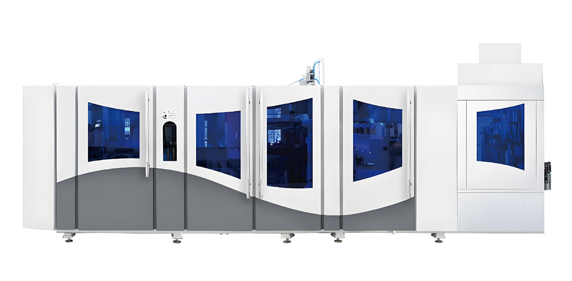
YuDa High Speed FGX Series

When a project’s contracted annual volume clears roughly 45 million bottles, the high-speed tier becomes the correct answer, and the YuDa FGX series is the platform built for that band. FGX machines are linear stretch blow molding systems delivering 8,000 to 15,000 bottles per hour, built around a single-mold speed of 2,500 to 3,000 bottles per hour and scaled by cavity count.

Three design decisions define the series. The first is a unique cam linking system that integrates mold opening, mold locking, and bottom mold elevation into one coordinated movement, which removes the sequencing dead time that limits conventional clamping architectures and allows the high single-mold cycle rate to be sustained rather than merely peaked. The second is a high-speed servo driving system, which replaces hydraulic actuation on the motion-critical axes, delivering repeatable stretch rod profiles and consuming energy in proportion to actual motion. The third is the compact heating oven with heater-to-preform distance minimized to 38.1 mm, delivering more than 30 percent heating electricity savings against conventional oven layouts.

The series is also modularized, so cavity blocks, oven sections, and transfer components can be serviced or reconfigured without disturbing the whole line, and it carries a remote monitoring system that lets engineers at the China headquarters read live PLC data and push abnormality feedback to the customer site. For an investor, that monitoring capability is a payback variable in its own right, because it compresses the diagnostic phase of any downtime event from days to hours.

Table 6 — YuDa FGX high speed series, typical configurations

Configuration	Cavities	Output	Bottle volume range	Neck diameter	Heating power	Air consumption	Operators required	Footprint
FGX 3-cavity	3	7,500–8,500 BPH	0.1–2.0 L	18–38 mm	66–78 kW	8–10 m³/min	1–2	24–28 m²
FGX 4-cavity	4	10,000–11,000 BPH	0.1–2.0 L	18–38 mm	88–104 kW	10–13 m³/min	2	30–34 m²
FGX 5-cavity	5	12,000–13,500 BPH	0.1–1.5 L	18–38 mm	110–130 kW	12–16 m³/min	2	34–40 m²
FGX 6-cavity	6	14,000–15,000 BPH	0.1–1.0 L	18–30 mm	132–156 kW	14–18 m³/min	2	40–46 m²

Output figures reference standard still water formats with a stable preform supply. Carbonated and hot-fill formats run at derated speed because of longer oven dwell and, for hot fill, heat-set mold conditioning. Air consumption is stated at working pressure and rises with bottle internal volume, which is why the 6-cavity configuration is specified toward smaller formats where cycle rate rather than air volume is the constraint.

Where the FGX Series Fits in a Payback Model

The FGX platform belongs in a payback model when three conditions hold simultaneously. Contracted annual volume must sit above roughly 45 million bottles per line. The SKU portfolio must be concentrated enough that changeovers do not consume the speed advantage — typically no more than four to six active formats sharing a common neck finish. And the utility infrastructure must be genuinely capable: a high-speed line starved of high-pressure air or served by an unstable chilled water circuit will underperform a standard-speed line every time.

Where those conditions hold, the FGX tier delivers the shortest payback available in PET bottle manufacturing, typically 14 to 22 months, because it combines the lowest unit conversion cost index with the lowest labor burden per bottle and the smallest footprint per unit of output. Where they do not hold, the same machine produces the longest payback in this guide, which is precisely why the sizing discipline described earlier matters more than the specification sheet.

YuDa Standard Speed and Semi-auto Series

Most PET bottle factory investments do not start in the high-speed tier, and they should not. The standard speed full automatic series covering 1,000 to 7,000 bottles per hour, and the semi-automatic series below it, together handle the majority of first plants, regional plants, and multi-format daily chemical operations. Both series are built on the same energy-saving heating philosophy and the same component selection discipline as the FGX platform, so a plant that starts standard and later adds high speed does not have to retrain its maintenance organization.

The full automatic standard series integrates preform feeding, orientation, heating, blowing, and discharge in a continuous line requiring two operators regardless of cavity count. The semi-automatic series separates preform loading and bottle unloading into manual steps, which lowers capital intensity substantially and allows delivery from stock, at the cost of a much higher labor burden per bottle. For enterprises entering the market with limited contracted volume, that trade is frequently correct, because the semi-automatic tier has the lowest break-even volume of any option and therefore the shortest path to positive cash flow at low utilization.

Table 7 — YuDa standard speed and semi-auto series, typical configurations

Configuration	Type	Cavities	Output	Bottle volume	Installed power	Air pressure	Footprint
Full automatic 1-cavity	Full automatic linear	1	1,000–1,500 BPH	0.1–5.0 L	26–34 kW	2.5–3.5 MPa	12–15 m²
Full automatic 2-cavity	Full automatic linear	2	2,000–3,000 BPH	0.1–2.0 L	40–52 kW	2.8–3.8 MPa	16–20 m²
Full automatic 4-cavity	Full automatic linear	4	4,000–5,000 BPH	0.1–2.0 L	68–86 kW	3.0–4.0 MPa	22–26 m²
Full automatic 6-cavity	Full automatic linear	6	6,000–7,000 BPH	0.1–1.5 L	96–120 kW	3.0–4.0 MPa	28–33 m²
Semi-auto 2-cavity	Semi-automatic	2	1,000–1,400 BPH	0.1–2.0 L	18–24 kW	2.5–3.0 MPa	8–10 m²
Semi-auto 4-cavity	Semi-automatic	4	1,800–2,400 BPH	0.1–1.5 L	28–36 kW	2.5–3.0 MPa	11–14 m²
Semi-auto large-volume	Semi-automatic	1	100–150 BPH	10–20 L	22–30 kW	2.0–2.5 MPa	9–12 m²

Application Industries Served by These Series

YuDa machines run across the full spread of PET packaging end markets, and the series selection follows the end market as much as the volume. In food and beverage, the dominant applications are still water in 350 mL to 1.5 L, carbonated soft drinks in 500 mL to 2.0 L with petaloid bases, juices and teas in hot-fill or aseptic-compatible formats, and dairy-adjacent drinks in small formats. In daily chemical, the applications are shampoo, liquid detergent, fabric softener, and surface cleaner bottles, generally in 250 mL to 2.0 L with wide-neck finishes and frequent format changes. In edible oil and condiments, the applications are 1.0 L to 5.0 L containers with handles or grip panels, typically running on standard speed machines because the volume per SKU is moderate. In bulk water, 10 to 20 L returnable and single-use containers run on dedicated semi-automatic large-volume equipment.

For projects that combine bottle production with filling in a single footprint, Wanplas also supplies linear blowing-filling-capping CombiBlock systems and full BFC lines that blow, fill, and cap drinking water in one integrated process. These reduce conveying, air conveyor infrastructure, and empty bottle handling entirely, which matters most where floor area is scarce or where empty bottle transport within the site would otherwise be a bottleneck.

Risk Register: 12 Risks and Mitigations

A payback model without a risk register is an average of a distribution nobody has drawn. The twelve risks below account for the large majority of the variance between projected and realized payback in PET bottle projects. Probability is graded Low, Medium, or High for a typical greenfield project in its first three years. Impact is graded by the number of months the risk typically adds to payback if it materializes without mitigation.

Table 8 — PET bottle plant risk register

#	Risk	Probability	Impact	Mitigation
1	Customer concentration above 50% of volume	High	Very High	Cap any single account at 35% of planned volume; qualify a second and third account before commissioning; write minimum-volume clauses with rolling notice periods into supply agreements
2	Preform supply price volatility	High	High	Index supply contracts to a published resin reference so movement passes through to customers; hold 3–5 weeks of preform inventory as a buffer; qualify two preform suppliers on identical specification
3	Power outage or tariff band increase	Medium	High	Specify low energy intensity equipment at purchase; install air recovery; negotiate time-of-use scheduling; size a generator for controlled shutdown rather than full production
4	Local overcapacity and price erosion	Medium	Very High	Survey installed capacity within the 300 km radius before committing; differentiate on format capability such as hot fill or wide neck rather than on price; secure contracted volume before adding lines
5	Mold delivery delay	Medium	Medium	Order molds in parallel with the machine, not after; obtain preform-to-bottle design validation before mold cutting; keep one universal water bottle mold available for early revenue
6	Technical staffing gap	High	High	Send two operators for factory training before shipment; document oven recipes per SKU; retain remote monitoring support; cross-train a second shift leader from month one
7	Quality rejection by brand owner	Medium	Very High	Agree the full test protocol before first article — top load, burst, drop, thermal stability, wall map, perpendicularity; buy the test equipment before the machine arrives, not after the first rejection
8	Delivery radius exceeding 300 km	Medium	High	Model unit logistics cost against radius before site selection; prefer in-house or in-park bottling models; consider a satellite line at the customer site rather than long-haul empty bottle freight
9	Seasonality swing of roughly 40% peak to trough	High	Medium	Balance a beverage portfolio with a counter-seasonal daily chemical or edible oil account; schedule annual maintenance and mold trials into the trough; plan shift patterns seasonally rather than annually
10	Regulatory change on recycled PET content	Medium	Medium	Validate the process window on preforms containing recycled content early; document intrinsic viscosity and acetaldehyde tolerance; specify oven control capable of handling wider material variation
11	Equipment obsolescence	Low	Medium	Choose modular platforms where cavity blocks and oven sections can be upgraded; prefer servo architectures with recipe storage; confirm long-term spare parts availability at purchase
12	Cash flow strain during ramp-up	High	High	Model the full ramp-up trough explicitly; hold working capital for at least five months of preform purchasing and payroll; negotiate shorter payment terms with early customers

How to Weight the Register

Not all twelve risks deserve equal management attention. Rank them by the product of probability and impact and the register collapses into a short priority list. Customer concentration, technical staffing gap, ramp-up cash strain, and preform volatility all combine High probability with High or Very High impact, and together they explain most realized payback overruns. Local overcapacity and brand-owner quality rejection are lower in probability but severe enough in impact that they justify pre-investment diligence rather than post-investment management.

The remaining risks are real but manageable through ordinary engineering discipline. Notably, equipment obsolescence — the risk investors most often ask about — is the lowest-ranked item on the list. PET stretch blow molding is a mature process, and a well-built servo line with modular architecture and available spare parts remains commercially competitive for well over a decade. The risk that actually destroys PET bottle projects is commercial, not technical.

Ramp-Up Curve: Month 1 to Month 12

The ramp-up curve is where a payback model meets reality, and it deserves its own line-by-line treatment rather than a single blended assumption. The table below describes a well-managed ramp for a full automatic line with a trained core crew, two initial SKUs, and one anchor customer already contracted. Cumulative cash position is indexed with the deepest trough set at minus 100 index points, so the figures show the shape of the cash curve rather than any absolute quantity.

Table 9 — Twelve-month ramp-up profile (cash trough = −100 index points)

Month	Expected utilization	Scrap rate	Cumulative cash position index	Key milestone
1	18%	9.0%	−42	Installation, commissioning, utility verification, first bottles blown
2	30%	6.5%	−72	Oven recipe development per SKU; first article samples submitted
3	42%	4.5%	−92	First article approval; wall map and top load validated; trial orders shipped
4	52%	3.4%	−100	Cash trough; second shift started; changeover procedure documented
5	60%	2.8%	−96	Anchor customer volume ramps; preventive maintenance schedule activated
6	66%	2.3%	−84	Second SKU stabilized; scrap analysis loop running weekly
7	71%	2.0%	−66	Third shift evaluated; second customer qualification begins
8	75%	1.8%	−44	Operating cash flow turns positive on a monthly basis
9	78%	1.6%	−20	Second customer first article approved; changeover time reduced
10	81%	1.5%	+6	Cumulative operating cash crosses zero; spare parts consumption normalizes
11	84%	1.4%	+34	Steady state approached; energy intensity benchmark established
12	86%	1.3%	+64	Full-year baseline set; second line decision evaluated on contracted volume

Reading the Ramp Correctly

Three features of this curve carry planning consequences. First, the cash trough occurs in month four, not month one. Working capital planning that covers only the installation period will run short exactly when the plant is consuming the most preform and generating the least revenue. Second, scrap falls faster than utilization rises. That is normal and desirable — process stabilization precedes volume, and a plant that pushes volume before stabilizing scrap converts material into rejects at an accelerating rate. Third, the crossover to cumulative positive operating cash happens around month ten in a well-managed ramp. A project that assumes month three is not aggressive; it is simply wrong, and the resulting financing gap is the single most common cause of distress in first-time PET bottle ventures.

A poorly managed ramp differs from this profile in a specific way: utilization tracks similarly but scrap plateaus near 4 to 5 percent instead of descending, because nobody owns the process. That single difference typically shifts the cash crossover from month ten to month sixteen or later, and adds nine to fifteen months to payback.

Product Mix Strategy

Product mix is the one variable an operator can change after the equipment is installed, which makes it the primary tool for improving a payback trajectory that has started badly. The four principal PET bottle categories differ sharply in margin band, equipment requirement, and changeover burden, and a deliberate blend usually outperforms any single category.

Table 10 — PET bottle product categories: margin, equipment requirement and changeover burden

Product category	Gross margin band	Equipment requirement	Changeover frequency	Typical preform weight	Strategic role
Still water, 350 mL–1.5 L	Low	High-speed line preferred; simple base; standard neck	Very Low	11–36 g	Volume base; absorbs fixed cost; secures utilization
Carbonated soft drink, 500 mL–2.0 L	Medium	Petaloid base molds; higher blow pressure; tighter wall control	Low	22–52 g	Margin upgrade on the same asset base
Hot-fill juice and tea	High	Heat-set molds, crystallized neck, elevated mold temperature control	Medium	28–48 g	Differentiator; limits competition from basic lines
Daily chemical and edible oil	High	Wide-neck tooling, handle or grip panel capability, standard speed adequate	High	18–95 g	Counter-seasonal balance; small-batch margin

Building a Blended Portfolio

The classic mistake is to chase the highest-margin category exclusively. A plant that fills its schedule with small-batch daily chemical work enjoys excellent per-bottle margin and terrible utilization, because changeovers consume the calendar. The classic opposite mistake is to run only water, which delivers superb utilization and margins so thin that a single tariff increase or a customer price renegotiation erases the return.

A robust blend anchors 55 to 70 percent of capacity on a high-volume water or carbonated contract that guarantees utilization, then layers 20 to 30 percent of hot-fill or specialty work for margin, and reserves 10 to 15 percent for small-batch daily chemical and edible oil business that balances the beverage season. Executed on the right equipment, this structure typically lifts blended gross margin by 4 to 9 percentage points against a water-only plant while holding utilization within 3 to 5 points of the water-only case.

Two operational preconditions make the blend work. Neck finish standardization across as many SKUs as possible allows format changes without changing grippers, transfer components, or preform feed tooling, which can cut changeover time by half. And scheduling discipline — grouping SKUs sharing a neck finish and running them in a fixed weekly sequence — converts changeover from a random disruption into a planned event that can be executed during a shift handover rather than during productive hours.

Make-or-Buy Preforms

Because preform and resin dominate the cost structure, every PET bottle investor eventually asks whether to bring preform injection in house. The answer depends far more on volume stability and technical capability than on the apparent margin available in the preform step, and getting it wrong in either direction is expensive.

Table 11 — Purchased preforms versus in-house preform injection

Dimension	Purchased preforms	In-house preform injection
Additional capital intensity index	0 (baseline)	+180 to +320 index points over a blow-only line
Quality controllability	Medium — depends on supplier discipline and lot consistency	High — intrinsic viscosity, acetaldehyde, moisture and gate quality controlled internally
Inventory burden	Medium — 3–5 weeks of preforms plus safety stock	High — resin, masterbatch, work in process and finished preforms
Minimum economic scale	Viable from the first million bottles	Generally above 60–80 million bottles per year on a stable neck finish set
SKU flexibility	High — new formats sourced without tooling investment	Low — each neck finish and gram weight requires its own preform mold
Technical staffing requirement	Blow molding process capability only	Adds injection molding, drying, hot runner and mold maintenance capability
Effect on payback period	Baseline	−4 to −9 months if the volume threshold is cleared and utilization holds above 80%; +8 to +18 months if it is not

The asymmetry in the final row is the whole argument. Integration rewards the plant that has already solved utilization and stabilized its neck finish portfolio, and punishes the plant that has not. A sensible sequencing rule is therefore to stay on purchased preforms through the first full year, use that year to consolidate neck finishes and build contracted volume, and revisit integration only when annual volume is above the threshold and at least 70 percent of it sits on two or fewer neck finishes.

One intermediate option deserves mention. Some plants negotiate a tolling arrangement in which they supply resin and a preform producer converts it, capturing part of the material margin without the capital or the technical burden. Where such an arrangement is available it usually delivers roughly a third of the integration benefit at close to none of the integration risk, and it is the correct first step for most projects.

Location and Logistics

Empty PET bottles are among the lowest-density freight in packaging. A standard trailer loaded with 500 mL bottles carries a payload that is mostly enclosed air, so freight cost per bottle rises steeply with distance while the value of the bottle stays constant. This physical fact makes location a first-order payback variable, not a facilities detail.

Table 12 — Delivery radius versus unit logistics cost index (baseline: under 50 km = 100)

Delivery radius	Unit logistics cost index	Share of conversion cost	Recommended supply model
Under 50 km	100 (baseline)	2–3%	Direct delivery; multiple daily drops feasible
50–150 km	145–185	3–5%	Direct delivery; consolidate into full loads
150–300 km	210–290	5–8%	Economic boundary; requires premium format or margin to justify
300–500 km	330–450	8–13%	Generally uneconomic for standard water; consider a satellite line
Above 500 km	Above 470	Above 13%	Not viable for empty bottles; supply preforms and blow at destination

The In-House Bottling Model

The logic of the table above pushes toward the shortest possible radius, and its logical endpoint is zero: install the blow molding line inside the customer’s bottling facility. In this model the bottle producer supplies bottles onto an air conveyor that feeds the filler directly, eliminating outbound freight, empty bottle warehousing, palletizing, depalletizing, and most bottle handling damage.

For the equipment investor, the in-house model changes several payback inputs at once. Logistics cost falls toward the floor of the range. Utilization becomes tightly coupled to the customer’s filling schedule, which is both a benefit and a concentration risk. Footprint becomes a binding constraint, because floor space inside an operating bottling plant is scarce and expensive, which favors high-speed lines with the smallest area per unit of output. And bottle handling damage, a quiet contributor to scrap in conventional supply chains, largely disappears.

The counterpart risk is item one on the register: an in-house line is by definition a single-customer asset. Projects that pursue this model should negotiate contract duration and minimum volume commitments proportionate to the equipment recovery period, and should confirm that the line can be relocated and reconfigured for a different neck finish if the relationship ends. Modular machine architecture is worth a premium in exactly this scenario.

Site Selection Checklist

• Customer geography first. Map contracted and prospective volume, then locate the plant at the weighted center of that demand, not at the cheapest available land.
• Electricity tariff band and reliability. Verify both the tariff structure and the historical outage record. A low tariff with frequent interruptions is worse than a medium tariff with stable supply, because every interruption produces an oven restart and a burst of scrap.
• Water and chilled water capacity. Mold cooling load scales with output; confirm cooling tower and chiller capacity for the eventual line count, not the first line.
• Compressed air room planning. Reserve space and electrical capacity for the high-pressure compressor and receiver at the final configuration. Retrofitting air capacity into a completed building is disproportionately expensive.
• Installed competing capacity within 300 km. Survey it honestly before committing. Regional overcapacity is the risk most frequently discovered after the machines are ordered.
• Preform supply proximity. Preforms are dense and travel efficiently, so preform supply can be sourced further afield than bottles can be delivered — but inbound reliability still deserves a second qualified source.

Requirement to Model Selection Guide

Machine selection should be derived from contracted annual volume, SKU structure, and margin ambition, in that order. The table below maps five common project profiles to a recommended YuDa configuration and an expected payback band. Payback bands assume a purchased-preform model, a medium energy tariff, disciplined scrap control below 2 percent after ramp, and contracted volume actually materializing as planned.

Table 13 — Requirement to model selection guide

Project profile	Annual volume target	Recommended YuDa configuration	Cavities	Suggested plant setup	Expected payback band
Market entry, single region, testing demand	~30 million bottles	1 × Full automatic standard speed, 6-cavity (6,000–7,000 BPH)	6	Two shifts; 2–3 SKUs on one neck finish; purchased preforms; one universal water mold plus one specialty mold	22–34 months
Stable contracted supply to regional beverage customers	~120 million bottles	2 × FGX 4-cavity high speed (10,000–11,000 BPH each)	4 + 4	Three shifts; 4–6 SKUs; air recovery fitted; second line staged 6–9 months after the first	17–26 months
Brand owner co-packing, high volume, tight quality protocol	~300 million bottles	3 × FGX 6-cavity (14,000–15,000 BPH each) plus 1 × full automatic 4-cavity for SKU flexibility	6 + 6 + 6 + 4	Three shifts continuous; in-park or in-house bottling model; full test laboratory; remote monitoring active on all lines	14–22 months
Multi-format daily chemical and edible oil, small batches	~18 million bottles across 15 or more SKUs	2 × Full automatic standard speed 2-cavity plus 1 × Semi-auto 4-cavity	2 + 2 + 4	Two shifts; wide-neck tooling set; quick-change mold carts; semi-auto reserved for trials and short runs	26–40 months
Bulk water, 10–20 L returnable containers	~2.5 million containers	1 × Semi-auto large-volume plus manual finishing station	1	One to two shifts; dedicated washing and filling downstream; minimal changeover	20–32 months

How to Adjust the Recommendation

Three adjustments turn this generic table into a project-specific answer. If contracted volume is below 70 percent of the target figure, step down one tier — an under-loaded high-speed line always underperforms a well-loaded standard line. If the SKU count exceeds eight active formats, add a dedicated standard-speed line for the tail rather than fragmenting the main line’s schedule. And if the energy tariff sits in the high band, the payback advantage of the high-speed tier widens, because its lower energy intensity index compounds against a higher tariff, so the volume threshold for stepping up falls by roughly 10 to 15 percent.

Financial Health Indicators to Track Monthly

A payback model is a forecast; the indicators below are the instruments that tell you whether the forecast is still true. Every one of them can be measured from data the plant already generates, and every one has a threshold beyond which management action is required rather than optional. Tracking these eight monthly, on one page, catches deterioration months before it appears in financial statements.

Table 14 — Monthly financial and operational health indicators

Indicator	Target band	Warning threshold	What it reveals
Overall equipment effectiveness	78–86%	Below 70% for two consecutive months	Combined availability, speed and quality performance; the master operating metric
Scrap rate	0.8–1.8%	Above 3.0%	Process control discipline and preform quality stability
Energy intensity, kWh per 1,000 bottles	Within 10% of the format benchmark	More than 20% above benchmark	Oven condition, air leakage, compressor control, lamp degradation
Labor hours per 1,000 bottles	0.25–0.55 on full automatic lines	Above 0.8	Staffing discipline, changeover burden, unplanned intervention frequency
On-time in-full delivery	Above 97%	Below 93%	Schedule reliability; leading indicator of customer attrition
Customer concentration ratio, largest account	Below 35%	Above 50%	Commercial fragility; the single strongest predictor of payback overrun
Days sales outstanding	30–55 days	Above 75 days	Working capital absorption; customer financial health
Preform inventory turns per year	10–17	Below 7	Purchasing discipline and demand forecast accuracy

Two of these indicators deserve special standing. Overall equipment effectiveness is the operational master metric because it aggregates the three loss families that matter and converts them into a single comparable number across lines, shifts, and formats. Customer concentration ratio is the commercial master metric because it is the only indicator on the list that predicts catastrophic rather than gradual deterioration. A plant can recover from a bad month on equipment effectiveness. It rarely recovers quickly from losing an account that represented 60 percent of its schedule.

A practical governance rhythm is a one-page monthly review covering all eight indicators with a trailing three-month trend, a mandatory root-cause note for any indicator crossing its warning threshold, and a quarterly re-run of the payback model with actual figures substituted for assumptions. That last step is the one most plants skip, and it is the one that turns a payback model from a financing document into a management tool.

How Equipment Choice Shortens Payback

Equipment choice affects payback through three channels, and it is worth separating them because they respond to different project conditions. The first channel is unit conversion cost: faster lines with modern ovens and servo motion produce each bottle with less energy and less labor. The second is capital intensity: faster lines require more capital to be recovered. The third, and most often neglected, is break-even volume: faster lines have a higher volume at which they begin to generate positive contribution.

These three channels produce a clean decision rule. Below roughly 45 million bottles of contracted annual volume per line, the standard speed full automatic tier delivers the shorter payback, because its lower capital intensity and lower break-even volume outweigh its higher unit conversion cost. Above roughly 70 million bottles per line, the high-speed FGX tier delivers the shorter payback decisively, because the unit conversion cost advantage of 12 to 18 index points now applies to enough bottles to overwhelm the capital difference. Between 45 and 70 million bottles, the answer depends on the confidence attached to the volume forecast: contracted volume favors stepping up, forecast volume favors staying down and adding a second line later.

The Staged Investment Approach

For most projects the highest-return strategy is not to pick a tier but to sequence them. Install a standard speed full automatic line sized to contracted volume. Use the first year to stabilize the process, consolidate neck finishes, qualify additional customers, and build a documented recipe library. Then add a high-speed FGX line against the volume that the first year proved, keeping the standard line for tail SKUs, trials, and seasonal overflow.

This sequence produces a shorter blended payback than either a single oversized line or a single undersized one, for three reasons. It avoids the utilization penalty of installing capacity ahead of demand. It preserves SKU flexibility, because the standard line absorbs the changeover-intensive work that would otherwise fragment the high-speed line’s schedule. And it de-risks the technical ramp, because the organization learns stretch blow molding on a more forgiving machine before it operates a machine where every minute of downtime costs three times as much output.

Specification Choices That Move the Number

Within any tier, a handful of specification decisions have a measurable payback effect and should be settled before the order rather than discussed as options.

• Oven geometry and lamp zoning. The dominant energy variable. A compact oven with minimized heater distance and zone-level control is worth 17 to 20 percent of total line electricity against conventional layouts.
• Servo versus hydraulic motion on stretch and clamping. Servo architecture improves repeatability, which lowers scrap, and consumes energy proportionally to motion. Both effects favor payback.
• Air recovery capability. Specify it at purchase. Retrofitting recovery piping and valving into a commissioned line costs more and delivers less.
• Neck finish range of the transfer and gripper system. A wider standard range reduces the tooling investment required for every future format and cuts changeover time.
• Remote monitoring and data access. Diagnostic speed is an availability variable. Being able to have the manufacturer’s engineers read live PLC data converts a multi-day fault investigation into a same-day resolution.
• Modularity of cavity blocks and oven sections. Determines whether the line can be upgraded or reconfigured rather than replaced when the product portfolio changes.

Service and Support

Service quality is a payback variable disguised as an after-sales topic. Every hour of unresolved downtime during ramp-up compounds directly into the cash trough described earlier, and every avoidable process error consumes preform inventory at the point where working capital is thinnest. YuDa, a Wanplas factory with more than twenty years of PET bottle blow molding specialization, more than twenty patents, and installations in over sixty countries, structures its support around that reality.

Testing before shipment. Every machine is run and verified before it leaves the factory, using the customer’s own preform and mold where supplied, so that the process window is established in China rather than discovered on site. This single step removes the most common cause of extended commissioning.

Installation and commissioning. Engineers support mechanical installation, utility connection verification, first blow, oven recipe development for the initial SKU set, and handover against an agreed acceptance protocol covering output rate, scrap rate, and bottle quality criteria.

Spare parts policy. Under the Wanplas brand promise, customers receive USD 500 free parts/year, alongside free replacement of parts damaged within the warranty period. For a plant in its first two years, that policy meaningfully reduces the unbudgeted maintenance spending that typically appears in months six through eighteen.

Operator and technician training. Training covers oven profiling, preform inspection, changeover procedure, stretch and pre-blow timing adjustment, mold temperature management, routine preventive maintenance, and fault diagnosis. Sending two people to the factory before shipment consistently outperforms training only on site, because the trainees learn on a machine that is not yet on a production schedule.

Remote monitoring and support. The remote monitoring system allows engineers at the China headquarters to read live PLC data and push abnormality feedback to the customer’s site. In practice this compresses diagnosis time dramatically and turns many potential service visits into a guided adjustment by the local team.

Open factory policy. Wanplas maintains an open factory policy across its network. Prospective buyers are welcome to visit, watch machines run, inspect build quality, and run trial production with their own preforms and molds before committing.

Capacity and configuration matching. Beyond machine supply, Wanplas can assist with a capacity and configuration matching assessment: taking a project’s contracted volume, SKU list, bottle drawings, neck finish set, utility conditions, and shift pattern, and returning a line configuration, cavity count, utility sizing, and realistic utilization and scrap assumptions for the payback model. Because these assumptions are the inputs that decide whether a project repays in fourteen months or fifty, having them reviewed by engineers who have commissioned lines in over sixty countries is worth considerably more than the review takes to arrange.

Frequently Asked Questions

What is a realistic payback period for a PET bottle factory?

For a project with contracted volume, utilization above 80 percent, scrap below 2 percent, and a medium energy tariff, payback typically falls between 14 and 26 months depending on equipment tier and product mix. Projects that stall in the 50 to 60 percent utilization band commonly stretch past 48 months, and projects below 45 percent utilization frequently never reach payback at all without a commercial restructuring. The range is wide because it is driven by operating variables, not by equipment quality.

Why is capacity utilization more important than machine speed?

Depreciation, facility overhead, most maintenance, and a large part of labor are fixed regardless of how many bottles the line produces. Utilization determines how many good bottles those fixed elements are spread across. Moving from 70 to 85 percent utilization lowers unit conversion cost by roughly 9 index points and shortens payback by 10 to 16 months, which typically exceeds the entire difference between two competing machine specifications. Machine speed only converts into payback if the order book fills it.

How much does scrap rate really affect the payback period?

More than any other operating variable except utilization. Preform and resin account for 62 to 72 percent of conversion cost, so every point of scrap destroys value from the largest line item, wastes the energy already invested in heating those preforms, consumes machine time, and reduces the output over which fixed cost is recovered. Running at 6 percent scrap instead of 1.5 percent typically adds 12 to 20 months to payback, and the fix is largely procedural rather than capital.

Should a first-time investor choose semi-automatic or high-speed equipment?

It depends entirely on contracted volume. Semi-automatic lines have the lowest capital intensity and the lowest break-even volume, which makes them the correct choice below roughly 8 million bottles per year, but their unit conversion cost index is around 163 against a high-speed baseline of 88, and they need three to four operators per shift. High-speed FGX lines invert that relationship above roughly 45 million bottles per year. Between those points, the standard speed full automatic tier is usually optimal.

Is it worth producing preforms in house?

Only after the blow molding operation is stable and volume is proven. In-house preform injection adds roughly 180 to 320 index points of capital intensity over a blow-only line and requires injection molding, drying, hot runner and mold maintenance capability that a blow-only plant does not have. Above roughly 60 to 80 million bottles per year on a consolidated neck finish set, it can shorten payback by 4 to 9 months. Below that threshold it typically extends payback by 8 to 18 months.

How far can empty PET bottles be shipped economically?

Empty bottles are extremely low-density freight, so trucks effectively carry air. Unit logistics cost roughly doubles between a 50 km radius and a 150 to 300 km radius, and roughly quadruples beyond 300 km. Most projects find the economic boundary between 200 and 300 km for standard water bottles. Beyond that, the correct structure is to ship preforms, which are dense and travel efficiently, and blow them at a satellite line near the filling point.

What energy consumption should a PET bottle plant expect?

For a servo-driven line with a modern oven, including the high-pressure compressor, expect roughly 15 to 22 kWh per 1,000 bottles on a 500 mL still water format, 30 to 40 kWh per 1,000 on 1.5 L, and 42 to 56 kWh per 1,000 on a 2.0 L carbonated format. Infrared heating accounts for 55 to 65 percent of that, high-pressure air for 25 to 35 percent, and servo and mechanical systems for the remainder. Older-generation lines with wide heater spacing typically run 25 to 45 percent above these bands.

Which risk most often destroys PET bottle projects?

Customer concentration. A plant where one account represents more than half of volume has financed its equipment against a single commercial relationship, and when that relationship ends, utilization steps down rather than declining gradually. Combined with ramp-up cash strain and technical staffing gaps, it explains most realized payback overruns. Equipment obsolescence, the risk investors most frequently ask about, ranks last on the register.

How long does a PET bottle plant take to reach steady-state operation?

A well-managed ramp reaches 70 percent utilization around month seven, 80 percent around month ten, and steady state near month twelve, with scrap declining from 8 to 10 percent in the commissioning month to below 1.5 percent by month ten. The cash trough occurs around month four, and cumulative operating cash typically turns positive around month ten. Working capital planning must cover that entire window, not just the installation period.

Conclusion

PET bottle manufacturing rewards operators who treat it as an operations business rather than an equipment purchase. The technology is mature and widely available; the machine you buy sets the ceiling on what is achievable, but the five operating variables — capacity utilization, scrap rate, energy tariff level, customer concentration, and product mix — determine where within that ceiling the plant actually lands. That is why two identical lines commissioned in the same month can return capital in fourteen months or in five years.

The practical discipline that separates the two outcomes is straightforward but rarely applied. Build the payback model on effective output rather than nameplate output, using an overall equipment effectiveness assumption you can defend from shift patterns, changeover counts, and scrap history. Recognize that material dominates the cost structure, so yield improvement outranks energy and labor programs. Model the ramp-up explicitly, including a cash trough around month four and a crossover around month ten. Size equipment against contracted volume, not against hoped-for volume, and step up tiers only when the volume that justifies the step is already committed. Maintain a live risk register, and watch customer concentration as closely as you watch scrap. And track eight indicators monthly against defined warning thresholds so that deterioration is visible while it is still correctable.

Where equipment does matter, it matters through three specific channels: energy intensity set by oven geometry and air system design, scrap driven by motion repeatability and process control, and availability determined by build quality, modularity, and how quickly a fault can be diagnosed. YuDa’s FGX high speed series, standard speed full automatic series, and semi-automatic series were developed across more than twenty years and over sixty export markets to address exactly those channels, with a compact 38.1 mm heater distance oven delivering over 30 percent heating energy savings, a cam linking clamp system sustaining high single-mold cycle rates, servo motion for repeatable stretch profiles, modular construction for serviceability, and remote monitoring that compresses diagnostic time when it matters most.

If you are evaluating a PET bottle factory investment, the most valuable next step is not a quotation — it is a configuration review. Send your contracted and forecast annual volume, bottle drawings and gram weights, neck finish set, SKU list, intended shift pattern, and your site’s electrical, compressed air and chilled water conditions. YuDa’s engineers, with Wanplas group support, will return a recommended line configuration and cavity count, realistic utilization and scrap assumptions for your payback model, utility sizing for the full build-out rather than the first line, and a staged investment path if one fits your volume profile better than a single purchase. You are also welcome to visit the factory under the Wanplas open factory policy, watch the machines run, and arrange a trial production run with your own preforms and molds before you commit to anything.